Nelder–Mead

1 Problem

Sometimes the multidimensional function is so difficult to evaluate that even expressing the 1^{\text{st}} derivative for gradient-based methods of finding optimum becomes an impossible task. In this case, we can only rely on the values of the function at each point. Or, in other words, on the 0 order oracle calls.

Let’s take, for instance, Mishra’s Bird function:

f(x,y) = \sin{y} \cdot e^{\left( 1 - \cos{x} \right)^2} + \cos{x} \cdot e^{\left( 1 - \sin{y} \right)^2} + (x - y)^2

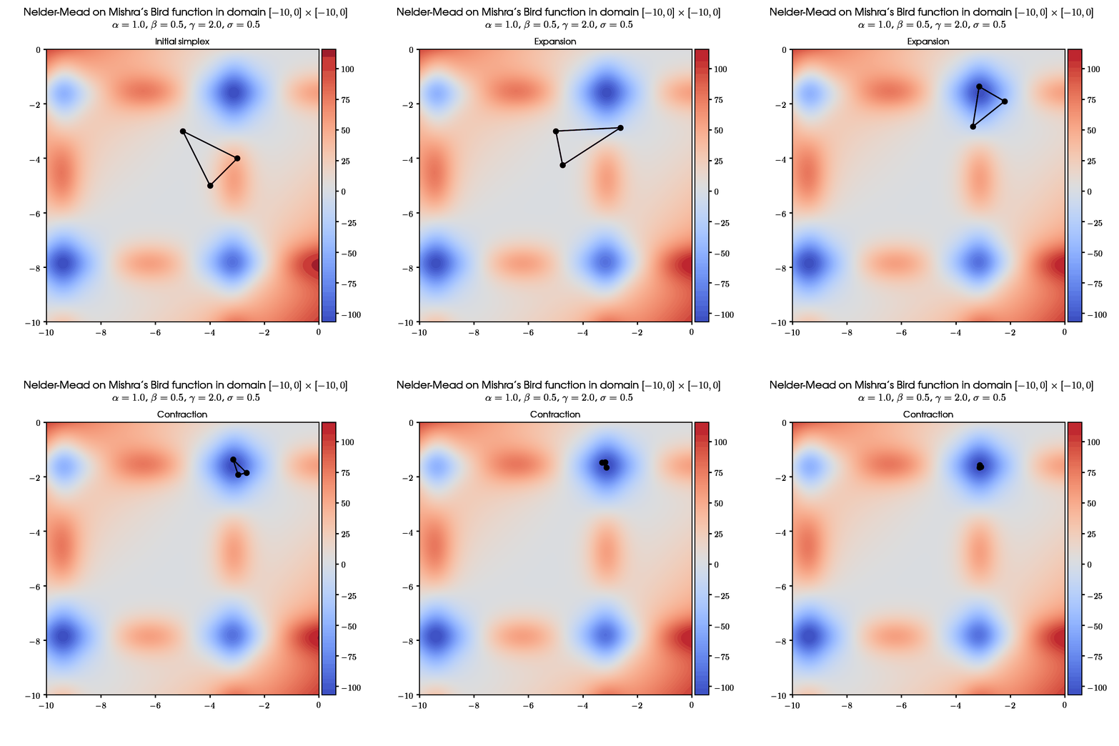
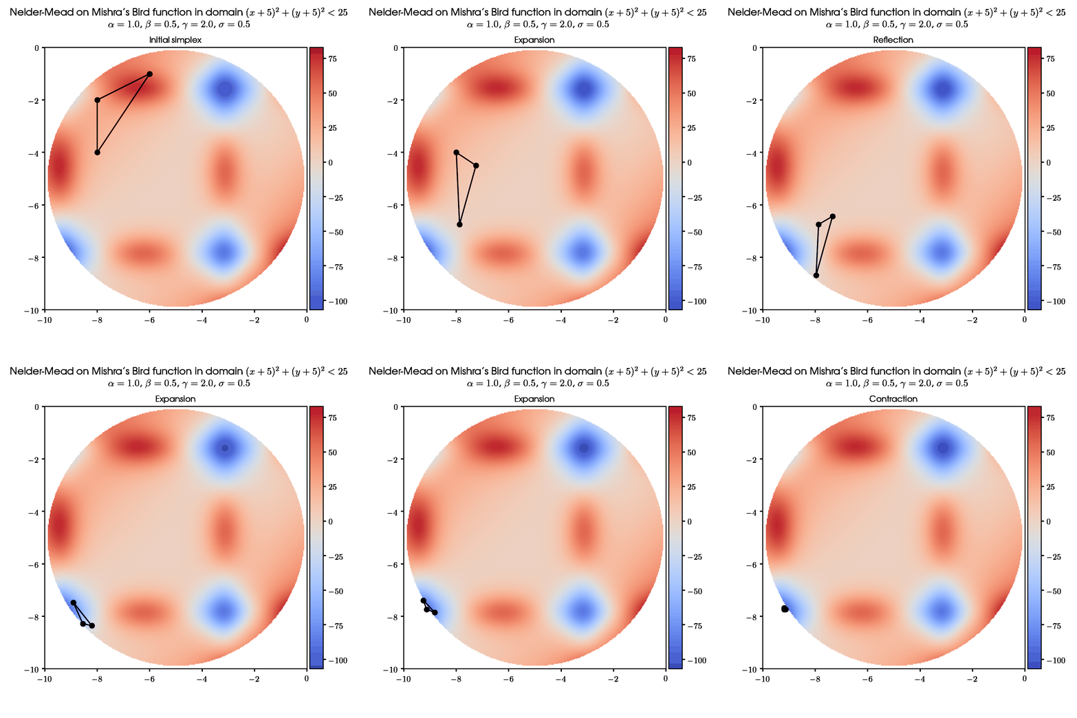
This function is usually subjected to the domain (x+5)^2 + (y+5)^2 < 25, but for the sake of picture beauty we will mainly use domain [-10; 0] \times [-10; 0].

2 Algorithm

2.2 Main idea

The algorithm maintains the set of test points in the form of simplex. For each point the function value is calculated and points are ordered accordingly. Depending on those values, the simplex exchanges the worst point of the set for the new one, which is closer to the local minimum. In some sense, the simplex is crawling to the minimal value in the domain.

The simplex movements finish when its sides become too small (termination condition by sides) or its area becomes too small (termination condition by area). I prefer the second condition, because it takes into account cases when simplex becomes degenerate (three or more vertices on one axis).

2.3 Steps of the algorithm

1. Ordering

Order vertices according to values in them:

f(x_1) \leqslant f(x_2) \leqslant \ldots \leqslant f(x_n) \leqslant f(x_{n+1})

Check the termination condition. Possible exit with solution x_{\min} = x_1.

2. Centroid calculation

x_o = \dfrac{\sum\limits_{k=1}^{n}{x_k}}{n}

3. Reflection

Calculate the reflected point x_r:

x_r = x_o + \alpha \left( x_o - x_{n+1} \right)

where \alpha – reflection coefficient, \alpha > 0. (If \alpha \leqslant 0, reflected point x_r will not overlap the centroid)

The next step is figured out according to the value of f(x_r) in dependency to values in points x_1 (best) and x_n (second worst):

f(x_r) < f(x_1): Go to step 4.
f(x_1) \leqslant f(x_r) < f(x_n): new simplex with x_{n+1} \rightarrow x_r. Go to step 1.
f(x_r) \geqslant f(x_n): Go to step 5.

4. Expansion

Calculate the expanded point x_e:

x_e = x_o + \gamma \left( x_r - x_o \right)

where \gamma – expansion coefficient, \gamma > 1. (If \gamma < 1, expanded point x_e will be contracted towards centroid, if \gamma = 1: x_e = x_r)

The next step is figured out according to the ratio between f(x_e) and f(x_r):

f(x_e) < f(x_r): new simplex with x_{n+1} \rightarrow x_e. Go to step 1.
f(x_e) > f(x_r): new simplex with x_{n+1} \rightarrow x_r. Go to step 1.

5. Contraction

Calculate the contracted point x_c:

x_c = x_o + \beta \left( x_{n+1} - x_o \right)

where \beta – contraction coefficient, 0 < \beta \leqslant 0.5. (If \beta > 0.5, contraction is insufficient, if \beta \leqslant 0, contracted point x_c overlaps the centroid)

The next step is figured out according to the ratio between f(x_c) and f(x_{n+1}):

f(x_c) < f(x_{n+1}): new simplex with x_{n+1} \rightarrow x_c. Go to step 1.
f(x_c) \geqslant f(x_{n+1}): Go to step 6.

6. Shrinkage

Replace all points of simplex x_i with new ones, except for the best point x_1:

x_i = x_1 + \sigma \left( x_i - x_1 \right)

where \sigma – shrinkage coefficient, 0 < \sigma < 1. (If \sigma \geqslant 1, shrinked point x_i overlaps the best point x_1, if \sigma \leqslant 0, shrinked point x_i becomes extended)

Go to step 1.

3 Examples

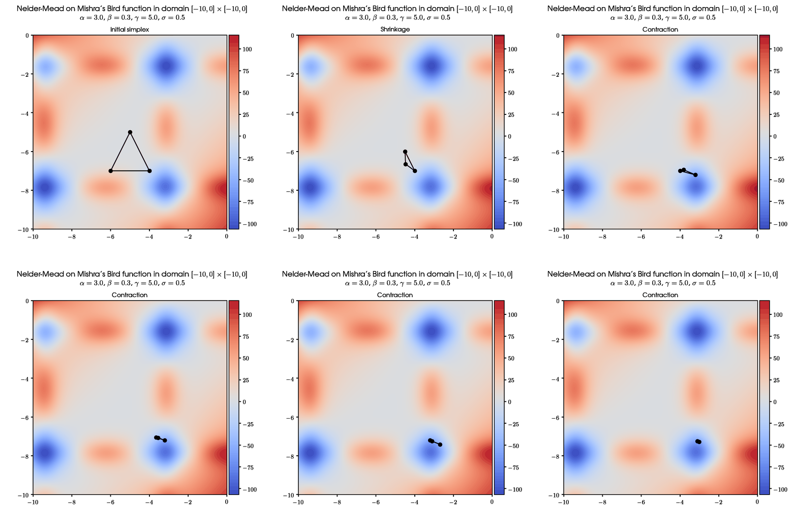
This algorithm, as any method in global optimization, is highly dependable on the initial conditions. For instance, if we use different initial simplex or different set of parameters \{ \alpha, \beta, \gamma, \sigma \} the resulting optimal point will differ.