Methods

1 General formulation

\begin{split} & \min_{x \in \mathbb{R}^n} f(x)\\ \text{s.t. } g_i(x) \leq& 0, \; i = 1,\ldots,m\\ h_j(x) =& 0, \; j = 1,\ldots,k\\ \end{split}

Some necessary or/and sufficient conditions are known (See Optimality conditions. KKT and Convex optimization problem.

• In fact, there might be very challenging to recognize the convenient form of optimization problem.
• Analytical solution of KKT could be inviable.

1.1 Iterative methods

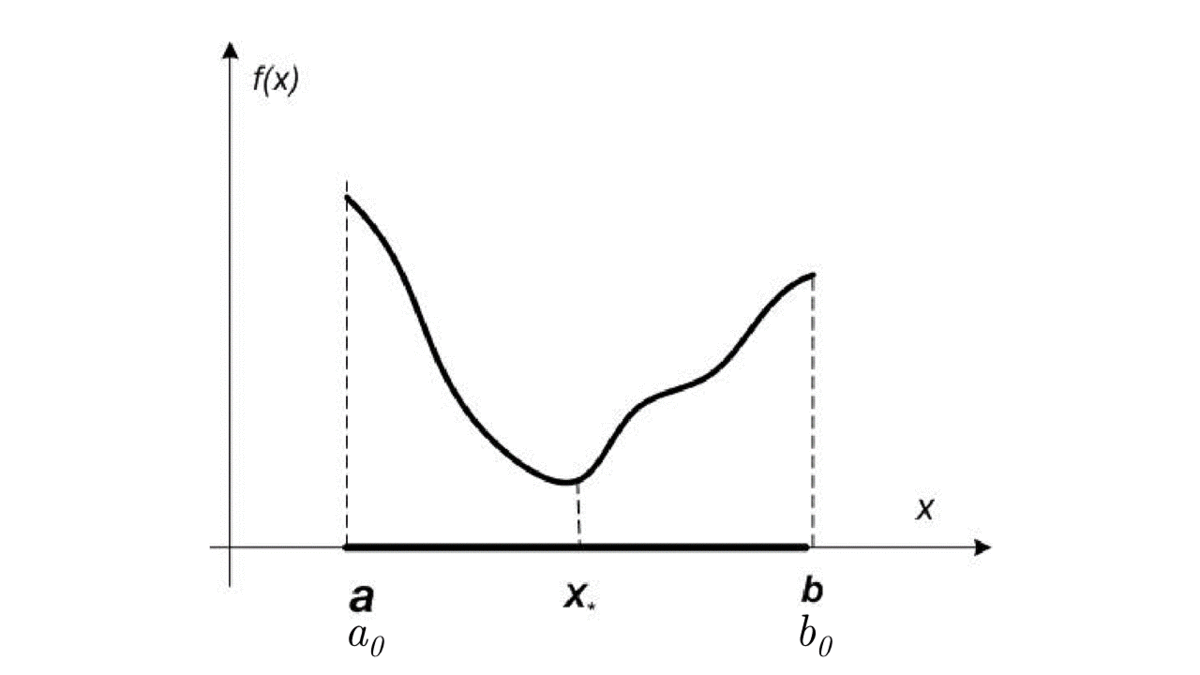
Typically, the methods generate an infinite sequence of approximate solutions

\{x_t\},

which for a finite number of steps (or better - time) converges to an optimal (at least one of the optimal) solution x_*.

Illustration of iterative method approaches to the solution x^*

def GeneralScheme(x, epsilon):
    while not StopCriterion(x, epsilon):
        OracleResponse = RequestOracle(x)
        x = NextPoint(x, OracleResponse)
    return x

1.2 Oracle conception

Depending on the maximum order of derivative available from the oracle we call the oracles as zero order, first order, second order oravle and etc.

2 Unsolvability of numerical optimization problem

In general, optimization problems are unsolvable. ¯\(ツ)/¯

Consider the following simple optimization problem of a function over unit cube:

\begin{split} & \min_{x \in \mathbb{R}^n} f(x)\\ \text{s.t. } & x \in \mathbb{C}^n \end{split}

We assume, that the objective function f (\cdot) : \mathbb{R}^n \to \mathbb{R} is Lipschitz continuous on \mathbb{B}^n:

| f (x) − f (y) | \leq L \| x − y \|_{\infty} \forall x,y \in \mathbb{C}^n,

with some constant L (Lipschitz constant). Here \mathbb{C}^n - the n-dimensional unit cube

\mathbb{C}^n = \{x \in \mathbb{R}^n \mid 0 \leq x_i \leq 1, i = 1, \ldots, n\}

Our goal is to find such \tilde{x}: \vert f(\tilde{x}) - f^*\vert \leq \varepsilon for some positive \varepsilon. Here f^* is the global minima of the problem. Uniform grid with p points on each dimension guarantees at least this quality:

\| \tilde{x} − x_* \|_{\infty} \leq \frac{1}{2p},

which means, that

|f (\tilde{x}) − f (x_*)| \leq \frac{L}{2p}

Our goal is to find the p for some \varepsilon. So, we need to sample \left(\frac{L}{2 \varepsilon}\right)^n points, since we need to measure function in p^n points. Doesn’t look scary, but if we’ll take L = 2, n = 11, \varepsilon = 0.01, computations on the modern personal computers will take 31,250,000 years.

2.1 Stopping rules

• Argument closeness:

  \| x_k - x_* \|_2 < \varepsilon

• Function value closeness:

  \| f_k - f^* \|_2 < \varepsilon

• Closeness to a critical point

  \| f'(x_k) \|_2 < \varepsilon

But x_* and f^* = f(x_*) are unknown!

Sometimes, we can use the trick:

\|x_{k+1} - x_k \| = \|x_{k+1} - x_k + x_* - x_* \| \leq \|x_{k+1} - x_* \| + \| x_k - x_* \| \leq 2\varepsilon

Note: it’s better to use relative changing of these values, i.e. \dfrac{\|x_{k+1} - x_k \|_2}{\| x_k \|_2}.

Example

Suppose, you are trying to estimate the vector x_{true} with some approximation x_{approx}. One can choose between two relative errors:

\dfrac{\|x_{approx} - x_{true}\|}{\|x_{approx}\|} \quad \dfrac{\|x_{approx} - x_{true}\|}{\|x_{true}\|}

If both x_{approx} and x_{true} are close to each other, then the difference between them is small, while if your approximation is far from the truth (say, x_{approx} = 10x_{true} or x_{approx} = 0.01 x_{true} they differ drastically).

2.2 Local nature of the methods

Illustration of the idea of locality in black-box optimization

3 Contents of the chapter