Neural network Lipschitz constant
1 Lipschitz constant and robustness to a small perturbation
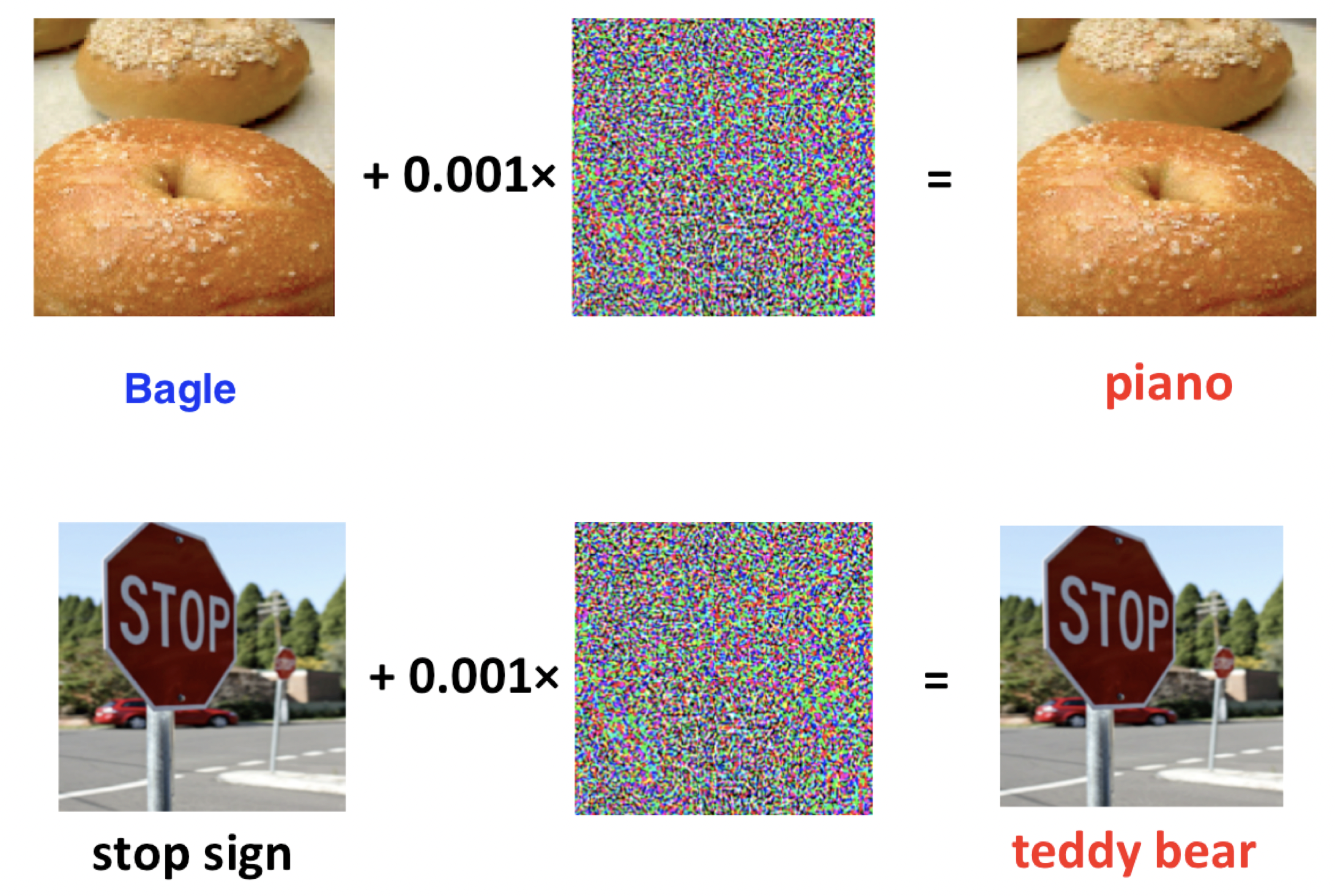
It was observed, that small perturbation in Neural Network input could lead to significant errors, i.e. misclassifications.

Lipschitz constant bounds the magnitude of the output of a function, so it cannot change drastically with a slight change in the input
\|\mathcal{NN}(image) - \mathcal{NN}(image+\varepsilon)\| \leq L_{\mathcal{NN}}\|\varepsilon\|
Note, that a variety of feed-forward neural networks could be represented as a series of linear transformations, followed by some nonlinear function (say, \text{ReLU }(x)):
\mathcal{NN}(x) = f_L \circ w_L \circ \ldots \circ f_1 \circ w_1 \circ x,
where L is the number of layers, f_i - non-linear activation function, w_i = W_i x + b_i - linear layer.
2 Estimating Lipschitz constant of a neural network
Therefore, we can bound the Lipschitz constant of a neural network:
L_{\mathcal{NN}} \leq L_{f_1} \ldots L_{f_L} L_{w_1} \ldots L_{w_L}
3 How to compute \|W\|_2?
Let W = U \Sigma V^T – SVD of the matrix W \in \mathbb{R}^{m \times n}. Then
\|W\|_2 = \sup_{x \ne 0} \frac{\| W x \|_2}{\| x \|_{2}} = \sigma_1(W) = \sqrt{\lambda_\text{max} (W^*W)}
For m = n, computing SVD is \mathcal{O}(n^3).
| n | 10 | 100 | 1000 | 5000 |
|---|---|---|---|---|
| Time | 38.7 µs | 3.04 ms | 717 ms | 1min 21s |
| Memory for W in fp32 | 0.4 KB | 40 KB | 4 MB | 95 MB |
Works only for small linear layers.
In this notebook we will try to estimate Lipschitz constant of some convolutional layer of a Neural Network.
4 Convolutional layer

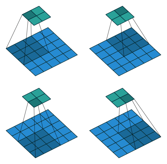
Suppose, that we have an input X and the convolutional layer C with the filter size k \times k. Here we assume, that p_1, p_2 - are the indices of pixels of the kernel, while q_1, q_2 are the indices of pixels of the output.
C \circ X = \sum_{p_1 = 0}^{k-1}\sum_{p_2 = 0}^{k-1} C_{p_1, p_2} X_{p_1 + q_1, p_2 + q_2}
While multichannel convolution could be written in the following form:
Y_j = \sum_{i = 1}^{m_{in}} C_{:, :, i, j} \circ X_{:, :, i},
where
- C \in \mathbb{R}^{k \times k \times m_{in} \times m_{out}} – convolution kernel
- k – filter size
- m_{in} – number of input channels (e.g., 3 for RGB)
- m_{out} – number of output channels.
It is easy to see, that the output of the multichannel convolution operation is linear w.r.t. the input X, which actually means, that one can write it as matvec:
\text{vec }(Y) = W \text{vec }(X)
It seems, that computing \|W\|_2 is almost impossible, isn’t it?
5 Power method for computing the largest singular value
Since we are interested in the largest singular value and
\|W\|_2 = \sigma_1(W) = \sqrt{\lambda_\text{max} (W^*W)}
we can apply the power method
x_{k+1} = \dfrac{W^T W x_k}{\|W^T W x_k\|_2}
\sigma_{k+1} = \dfrac{W x_{k+1}}{\|x_{k+1}\|_2}
6 Code
Open In Colab{: .btn }
7 References
- Maxim Rakhuba’s lecture on Matrix and tensor methods in ML.